How to Read T Test Results in R
How to Do a T-test in R: Calculation and Reporting
This article describes how to do a t-test in R (or in Rstudio). You lot will acquire how to:
- Perform a t-test in R using the following functions :
-
t_test()[rstatix package]: a wrapper around the R base officet.test(). The effect is a information frame, which can exist hands added to a plot using theggpubrR package. -
t.test()[stats package]: R base function to conduct a t-examination.
-
- Interpret and report the t-test
- Add p-values and significance levels to a plot
- Calculate and report the t-test effect size using Cohen's d. The
dstatistic redefines the divergence in means as the number of standard deviations that separates those means. T-test conventional upshot sizes, proposed by Cohen, are: 0.2 (pocket-sized effect), 0.5 (moderate effect) and 0.8 (large issue) (Cohen 1998).
We volition provide examples of R lawmaking to run the different types of t-test in R, including the:
- 1-sample t-examination
- two-sample t-test (also known equally independent t-examination or unpaired t-test)
- paired t-exam (also known as dependent t-test or matched pairs t examination)
Contents:
- Prerequisites
- One-sample t-test
- Demo data
- Summary statistics
- Calculation
- Estimation
- Effect size
- Reporting
- Ii-sample t-exam
- Demo information
- Summary statistics
- Adding
- Interpretation
- Effect size
- Cohen's d for Student t-test
- Cohen'due south d for Welch t-examination
- Report
- Paired t-test
- Demo data
- Summary statistics
- Adding
- Interpretation
- Outcome size
- Report
- Summary
- References
Related Book
Practical Statistics in R II - Comparing Groups: Numerical Variables
Prerequisites
Make sure you accept installed the following R packages:
-
tidyversefor information manipulation and visualization -
ggpubrfor creating hands publication fix plots -
rstatixprovides pipe-friendly R functions for easy statistical analyses. -
datarium: contains required data sets for this chapter.
Start by loading the following required packages:
library(tidyverse) library(ggpubr) library(rstatix) One-sample t-test
Demo data
Demo dataset: mice [in datarium bundle]. Contains the weight of 10 mice:
# Load and audit the data data(mice, packet = "datarium") head(mice, 3) ## # A tibble: 3 x 2 ## name weight ## <chr> <dbl> ## i M_1 eighteen.nine ## 2 M_2 19.v ## 3 M_3 23.ane We desire to know, whether the average weight of the mice differs from 25g (two-tailed test)?
Summary statistics
Compute some summary statistics: count (number of subjects), mean and sd (standard departure)
mice %>% get_summary_stats(weight, type = "mean_sd") ## # A tibble: ane x 4 ## variable n mean sd ## <chr> <dbl> <dbl> <dbl> ## 1 weight 10 20.one one.90 Calculation
Using the R base office
res <- t.examination(mice$weight, mu = 25) res ## ## One Sample t-test ## ## data: mice$weight ## t = -viii, df = ix, p-value = 2e-05 ## alternative hypothesis: true mean is not equal to 25 ## 95 percent confidence interval: ## 18.8 21.5 ## sample estimates: ## mean of x ## xx.1 In the result above :
-
tis the t-exam statistic value (t = -8.105), -
dfis the degrees of freedom (df= ix), -
p-valueis the significance level of the t-exam (p-value = 1.99510^{-five}). -
conf.intis the confidence interval of the mean at 95% (conf.int = [18.7835, 21.4965]); -
sample estimatesis the hateful value of the sample (hateful = 20.14).
Using the rstatix package
We'll utilise the piping-friendly t_test() function [rstatix bundle], a wrapper effectually the R base office t.test(). The results tin be hands added to a plot using the ggpubr R packet.
stat.test <- mice %>% t_test(weight ~ one, mu = 25) stat.examination ## # A tibble: i ten seven ## .y. group1 group2 north statistic df p ## * <chr> <chr> <chr> <int> <dbl> <dbl> <dbl> ## 1 weight 1 naught model 10 -viii.x nine 0.00002 The results above testify the post-obit components:
-
.y.: the effect variable used in the test. -
group1,group2: generally, the compared groups in the pairwise tests. Here, we have null model (one-sample exam). -
statistic: test statistic (t-value) used to compute the p-value. -
df: degrees of freedom. -
p: p-value.
You can obtain a detailed effect by specifying the option detailed = TRUE in the function t_test().
mice %>% t_test(weight ~ one, mu = 25, detailed = True) ## # A tibble: i x 12 ## judge .y. group1 group2 n statistic p df conf.low conf.high method alternative ## * <dbl> <chr> <chr> <chr> <int> <dbl> <dbl> <dbl> <dbl> <dbl> <chr> <chr> ## 1 20.1 weight 1 null model 10 -viii.10 0.00002 9 xviii.8 21.5 T-exam two.sided Estimation
The p-value of the test is 210^{-5}, which is less than the significance level alpha = 0.05. We tin conclude that the mean weight of the mice is significantly different from 25g with a p-value = 210^{-5}.
Upshot size
To calculate an effect size, chosen Cohen'southward d, for the one-sample t-exam yous need to divide the mean difference past the standard departure of the difference, every bit shown below. Note that, here: sd(x-mu) = sd(x).
Cohen's d formula:
\[
d = \frac{yard-\mu}{s}
\]
- \(m\) is the sample hateful
- \(s\) is the sample standard departure with \(n-i\) degrees of freedom
- \(\mu\) is the theoretical mean against which the mean of our sample is compared (default value is mu = 0).
Adding:
mice %>% cohens_d(weight ~ 1, mu = 25) ## # A tibble: 1 x 6 ## .y. group1 group2 effsize due north magnitude ## * <chr> <chr> <chr> <dbl> <int> <ord> ## 1 weight 1 zilch model 10.6 10 big Call up that, t-exam conventional effect sizes, proposed by Cohen J. (1998), are: 0.2 (small effect), 0.5 (moderate issue) and 0.8 (large effect) (Cohen 1998). As the effect size, d, is 2.56 you can conclude that there is a large effect.
Reporting
We could report the result equally follow:
A one-sample t-test was computed to determine whether the recruited mice average weight was different to the population normal mean weight (25g).
The measured mice mean weight (20.fourteen +/- 1.94) was statistically significantly lower than the population normal mean weight 25 (t(9) = -viii.1, p < 0.0001, d = two.56); where t(9) is shorthand notation for a t-statistic that has 9 degrees of freedom.
The results tin can exist visualized using either a box plot or a density plot.
Box Plot
Create a boxplot to visualize the distribution of mice weights. Add together besides jittered points to evidence individual observations. The big dot represents the hateful bespeak.
# Create the box-plot bxp <- ggboxplot( mice$weight, width = 0.5, add = c("hateful", "jitter"), ylab = "Weight (thousand)", xlab = Imitation ) # Add significance levels bxp + labs(subtitle = get_test_label(stat.test, detailed = TRUE)) 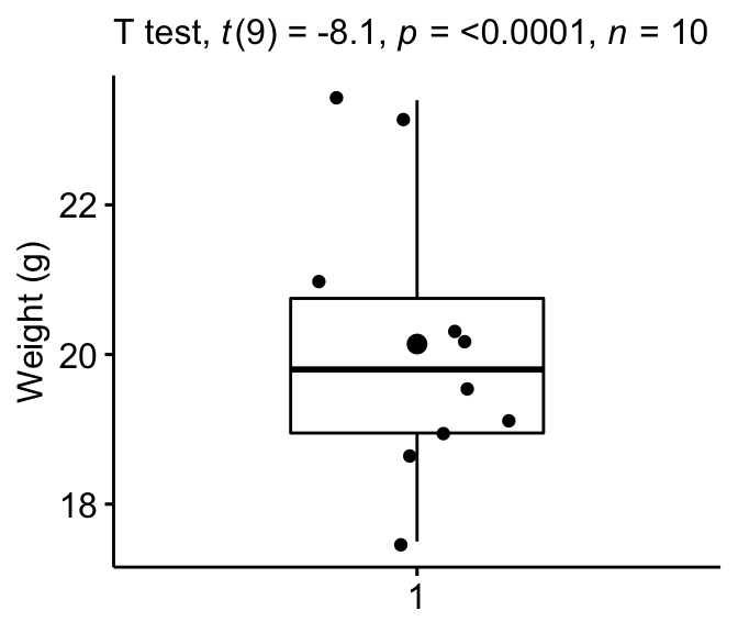
Density plot
Create a density plot with p-value:
- Red line corresponds to the observed hateful
- Blue line corresponds to the theoretical hateful
ggdensity(mice, x = "weight", rug = Truthful, fill = "lightgray") + scale_x_continuous(limits = c(fifteen, 27)) + stat_central_tendency(type = "mean", color = "red", linetype = "dashed") + geom_vline(xintercept = 25, colour = "bluish", linetype = "dashed") + labs(subtitle = get_test_label(stat.examination, detailed = TRUE)) 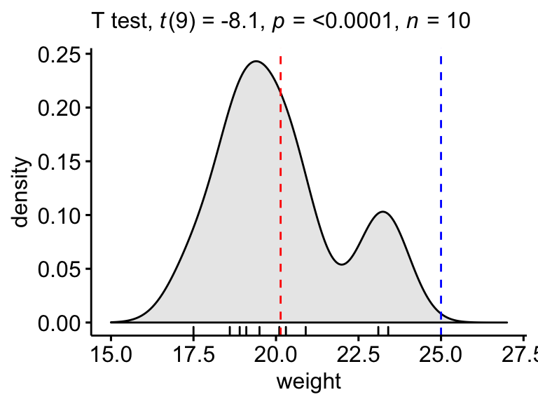
Two-sample t-examination
The ii-sample t-test is as well known as the independent t-test. The independent samples t-test comes in two different forms:
- the standard Student'due south t-test, which assumes that the variance of the two groups are equal.
- the Welch's t-test, which is less restrictive compared to the original Pupil's test. This is the test where you do not assume that the variance is the aforementioned in the ii groups, which results in the fractional degrees of liberty.
The two methods requite very similar results unless both the grouping sizes and the standard deviations are very unlike.
Demo data
Demo dataset: genderweight [in datarium package] containing the weight of 40 individuals (xx women and 20 men).
Load the data and show some random rows by groups:
# Load the data data("genderweight", package = "datarium") # Testify a sample of the information by group set.seed(123) genderweight %>% sample_n_by(group, size = 2) ## # A tibble: 4 x iii ## id group weight ## <fct> <fct> <dbl> ## 1 6 F 65.0 ## 2 xv F 65.ix ## 3 29 1000 88.ix ## 4 37 Thou 77.0 We want to know, whether the average weights are different between groups.
Summary statistics
Compute some summary statistics by groups: mean and sd (standard deviation)
genderweight %>% group_by(group) %>% get_summary_stats(weight, type = "mean_sd") ## # A tibble: two x 5 ## group variable due north mean sd ## <fct> <chr> <dbl> <dbl> <dbl> ## i F weight xx 63.5 2.03 ## 2 G weight 20 85.8 4.35 Adding
Recall that, by default, R computes the Welch t-examination, which is the safer i. This is the exam where you practice not assume that the variance is the same in the 2 groups, which results in the fractional degrees of liberty. If you desire to presume the equality of variances (Student t-test), specify the choice var.equal = TRUE.
Using the R base of operations role
res <- t.test(weight ~ group, data = genderweight) res ## ## Welch 2 Sample t-test ## ## data: weight by grouping ## t = -xx, df = 30, p-value <2e-16 ## alternative hypothesis: truthful difference in means is not equal to 0 ## 95 percent confidence interval: ## -24.5 -20.1 ## sample estimates: ## mean in group F hateful in group M ## 63.5 85.8 In the issue in a higher place :
-
tis the t-test statistic value (t = -twenty.79), -
dfis the degrees of freedom (df= 26.872), -
p-valueis the significance level of the t-test (p-value = iv.29810^{-xviii}). -
conf.intis the confidence interval of the means deviation at 95% (conf.int = [-24.5314, -xx.1235]); -
sample estimatesis the mean value of the sample (mean = 63.499, 85.826).
Using the rstatix package
stat.exam <- genderweight %>% t_test(weight ~ group) %>% add_significance() stat.exam ## # A tibble: one x 9 ## .y. group1 group2 n1 n2 statistic df p p.signif ## <chr> <chr> <chr> <int> <int> <dbl> <dbl> <dbl> <chr> ## 1 weight F Thousand xx 20 -twenty.8 26.ix iv.30e-18 **** The results higher up bear witness the following components:
-
.y.: the y variable used in the exam. -
group1,group2: the compared groups in the pairwise tests. -
statistic: Test statistic used to compute the p-value. -
df: degrees of freedom. -
p: p-value.
Annotation that, you can obtain a detailed issue past specifying the option detailed = TRUE.
genderweight %>% t_test(weight ~ group, detailed = TRUE) %>% add_significance() ## # A tibble: 1 x xvi ## judge estimate1 estimate2 .y. group1 group2 n1 n2 statistic p df conf.low conf.high method alternative p.signif ## <dbl> <dbl> <dbl> <chr> <chr> <chr> <int> <int> <dbl> <dbl> <dbl> <dbl> <dbl> <chr> <chr> <chr> ## ane -22.3 63.5 85.8 weight F M twenty 20 -20.8 4.30e-18 26.9 -24.5 -twenty.one T-test two.sided **** Interpretation
The p-value of the test is iv.310^{-18}, which is less than the significance level alpha = 0.05. We can conclude that men's average weight is significantly different from women's boilerplate weight with a p-value = four.310^{-eighteen}.
Consequence size
Cohen'southward d for Pupil t-test
There are multiple version of Cohen's d for Educatee t-test. The nearly usually used version of the Student t-test effect size, comparing ii groups (\(A\) and \(B\)), is calculated by dividing the mean divergence betwixt the groups past the pooled standard divergence.
Cohen'southward d formula:
\[
d = \frac{m_A - m_B}{SD_{pooled}}
\]
where,
- \(m_A\) and \(m_B\) represent the hateful value of the grouping A and B, respectively.
- \(n_A\) and \(n_B\) stand for the sizes of the grouping A and B, respectively.
- \(SD_{pooled}\) is an estimator of the pooled standard difference of the 2 groups. It tin can be calculated every bit follow :
\[
SD_{pooled} = \sqrt{\frac{\sum{(x-m_A)^2}+\sum{(x-m_B)^2}}{n_A+n_B-two}}
\]
Adding. If the pick var.equal = Truthful, then the pooled SD is used when computing the Cohen's d.
genderweight %>% cohens_d(weight ~ grouping, var.equal = TRUE) ## # A tibble: 1 x 7 ## .y. group1 group2 effsize n1 n2 magnitude ## * <chr> <chr> <chr> <dbl> <int> <int> <ord> ## 1 weight F M -6.57 20 20 big There is a large issue size, d = 6.57.
Notation that, for small sample size (< 50), the Cohen's d tends to over-inflate results. At that place exists a Hedge's Corrected version of the Cohen'southward d (Hedges and Olkin 1985), which reduces effect sizes for small samples by a few pct points. The correction is introduced by multiplying the usual value of d by (N-3)/(N-2.25) (for unpaired t-test) and past (n1-ii)/(n1-ane.25) for paired t-test; where Northward is the total size of the two groups being compared (North = n1 + n2).
Cohen's d for Welch t-test
The Welch test is a variant of t-test used when the equality of variance can't be assumed. The outcome size tin exist computed by dividing the mean difference between the groups past the "averaged" standard deviation.
Cohen's d formula:
\[
d = \frac{m_A - m_B}{\sqrt{(Var_1 + Var_2)/2}}
\]
where,
- \(m_A\) and \(m_B\) represent the mean value of the group A and B, respectively.
- \(Var_1\) and \(Var_2\) are the variance of the two groups.
Calculation:
genderweight %>% cohens_d(weight ~ group, var.equal = Faux) ## # A tibble: 1 x 7 ## .y. group1 group2 effsize n1 n2 magnitude ## * <chr> <chr> <chr> <dbl> <int> <int> <ord> ## one weight F Thou -six.57 20 20 large Note that, when grouping sizes are equal and group variances are homogeneous, Cohen'south d for the standard Pupil and Welch t-tests are identical.
Report
Nosotros could written report the effect as follow:
The mean weight in female person grouping was 63.5 (SD = two.03), whereas the mean in male group was 85.8 (SD = iv.3). A Welch two-samples t-test showed that the difference was statistically pregnant, t(26.nine) = -20.8, p < 0.0001, d = 6.57; where, t(26.9) is shorthand notation for a Welch t-statistic that has 26.9 degrees of liberty.
Visualize the results:
# Create a box-plot bxp <- ggboxplot( genderweight, x = "grouping", y = "weight", ylab = "Weight", xlab = "Groups", add = "jitter" ) # Add p-value and significance levels stat.exam <- stat.test %>% add_xy_position(x = "group") bxp + stat_pvalue_manual(stat.test, tip.length = 0) + labs(subtitle = get_test_label(stat.test, detailed = True)) 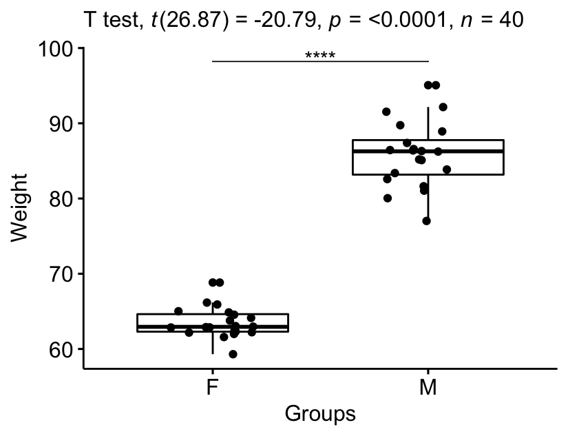
Paired t-test
Demo data
Here, we'll use a demo dataset mice2 [datarium package], which contains the weight of 10 mice earlier and after the treatment.
# Wide format data("mice2", package = "datarium") head(mice2, 3) ## id before afterwards ## 1 1 187 430 ## 2 2 194 404 ## 3 3 232 406 # Transform into long data: # gather the before and after values in the same column mice2.long <- mice2 %>% gather(key = "group", value = "weight", before, after) head(mice2.long, 3) ## id group weight ## 1 i before 187 ## two 2 earlier 194 ## 3 iii before 232 We want to know, if at that place is any meaning difference in the mean weights after handling?
Summary statistics
Compute some summary statistics (mean and sd) by groups:
mice2.long %>% group_by(group) %>% get_summary_stats(weight, type = "mean_sd") ## # A tibble: two 10 five ## group variable n mean sd ## <chr> <chr> <dbl> <dbl> <dbl> ## 1 after weight ten 400. 30.ane ## two before weight 10 201. 20.0 Calculation
Using the R base of operations function
res <- t.test(weight ~ grouping, data = mice2.long, paired = TRUE) res In the result above :
-
tis the t-test statistic value (t = -20.79), -
dfis the degrees of liberty (df= 26.872), -
p-valueis the significance level of the t-test (p-value = four.29810^{-18}). -
conf.intis the confidence interval of the mean of the differences at 95% (conf.int = [-24.5314, -20.1235]); -
sample estimatesis the mean of the differences (hateful = 63.499, 85.826).
Using the rstatix package
stat.exam <- mice2.long %>% t_test(weight ~ grouping, paired = True) %>% add_significance() stat.test ## # A tibble: 1 10 9 ## .y. group1 group2 n1 n2 statistic df p p.signif ## <chr> <chr> <chr> <int> <int> <dbl> <dbl> <dbl> <chr> ## 1 weight afterward before 10 10 25.5 ix 0.00000000104 **** The results above evidence the following components:
-
.y.: the y variable used in the test. -
group1,group2: the compared groups in the pairwise tests. -
statistic: Test statistic used to compute the p-value. -
df: degrees of freedom. -
p: p-value.
Notation that, you can obtain a detailed result by specifying the pick detailed = True.
mice2.long %>% t_test(weight ~ group, paired = TRUE, detailed = True) %>% add_significance() ## # A tibble: 1 ten 14 ## gauge .y. group1 group2 n1 n2 statistic p df conf.depression conf.high method alternative p.signif ## <dbl> <chr> <chr> <chr> <int> <int> <dbl> <dbl> <dbl> <dbl> <dbl> <chr> <chr> <chr> ## ane 199. weight after before x 10 25.five 0.00000000104 9 182. 217. T-examination two.sided **** Interpretation
The p-value of the test is 1.0410^{-9}, which is less than the significance level blastoff = 0.05. We can then turn down null hypothesis and conclude that the boilerplate weight of the mice before treatment is significantly different from the boilerplate weight afterwards treatment with a p-value = 1.0410^{-nine}.
Effect size
The effect size for a paired-samples t-exam tin can be calculated by dividing the mean deviation past the standard difference of the difference, every bit shown below.
Cohen's d formula:
\[
d = \frac{mean_D}{SD_D}
\]
Where D is the differences of the paired samples values.
Calculation:
mice2.long %>% cohens_d(weight ~ group, paired = Truthful) ## # A tibble: i x 7 ## .y. group1 group2 effsize n1 n2 magnitude ## * <chr> <chr> <chr> <dbl> <int> <int> <ord> ## 1 weight after before 8.08 10 10 big There is a large effect size, Cohen'south d = 8.07.
Report
Nosotros could report the consequence equally follow: The average weight of mice was significantly increased after treatment, t(9) = 25.5, p < 0.0001, d = 8.07.
Visualize the results:
# Create a box plot bxp <- ggpaired(mice2.long, x = "group", y = "weight", order = c("earlier", "later on"), ylab = "Weight", xlab = "Groups") # Add together p-value and significance levels stat.exam <- stat.test %>% add_xy_position(x = "group") bxp + stat_pvalue_manual(stat.test, tip.length = 0) + labs(subtitle = get_test_label(stat.test, detailed= True)) 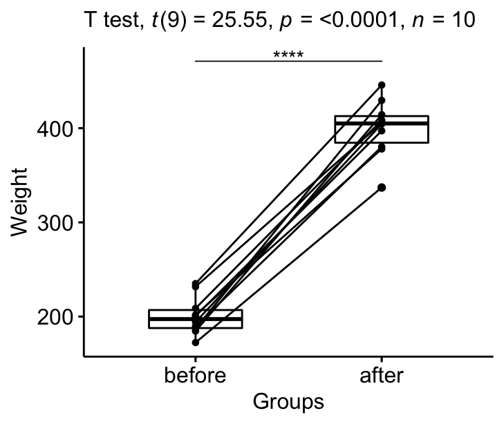
Summary
This commodity shows how to conduct a t-test in R/Rstudio using 2 different means: the R base of operations office t.exam() and the t_test() role in the rstatix package. Nosotros also draw how to interpret and report the t-test results.
References
Cohen, J. 1998. Statistical Power Analysis for the Behavioral Sciences. 2d ed. Hillsdale, NJ: Lawrence Erlbaum Associates.
Hedges, Larry, and Ingram Olkin. 1985. "Statistical Methods in Meta-Assay." In Stat Med. Vol. 20. doi:10.2307/1164953.
Recommended for y'all
This section contains best data science and cocky-evolution resources to help y'all on your path.
Version:  Français
Source: https://www.datanovia.com/en/lessons/how-to-do-a-t-test-in-r-calculation-and-reporting/
0 Response to "How to Read T Test Results in R"
Post a Comment